
First published on scylladb.com on April 22, 2021.
Many of us have heard of Coordinated Omission (CO), but few understand what it means, how to mitigate the problem, and why anyone should bother. Or, perhaps, this is the first time you have heard of the term. So let’s begin with a definition of what it is and why you should be concerned about it in your benchmarking.
The shortest and most elegant explanation of COs I have ever seen was from Daniel Compton in Artillery #721.
Coordinated omission is a term coined by Gil Tene to describe the phenomenon when the measuring system inadvertently coordinates with the system being measured in a way that avoids measuring outliers.
To that, I would add: …and misses sending requests.
To describe it in layman’s terms, let’s imagine a coffee-fueled office. Each hour a worker has to make a coffee run to the local coffee shop. But what if there’s a road closure in the middle of the day? You have to wait a few hours to go on that run. Not only is that hour’s particular coffee runner late, but all the other coffee runs get backed up for hours behind that. Sure, it takes the same amount of time to get the coffee once the road finally opens, but if you don’t measure that gap caused by the road closure, you’re missing measuring the total delay in getting your team their coffee. And, of course, in the meanwhile you will be woefully undercaffeinated.
CO is a concern because if your benchmark or a measuring system is suffering from it, then the results will be rendered useless or at least will look a lot more positive than they actually are.
Over the last 10 years, most benchmark implementations have been corrected by their authors to account for coordinated omission. Even so, using benchmark tools still requires knowledge to produce meaningful results and to spot any CO occurring. By default they do NOT respect CO.
Let’s take a look at how Coordinated Omission arises and how to solve it.
The Problem
Let’s consider the most popular use case: measuring performance characteristics of the web application – a system that consists of a client that makes requests to the database. There are different parameters we can look at. What are we interested in?
The first step in measuring the performance of a system is understanding what kind of system you’re dealing with.
For our purposes, there are basically two kinds of systems: open model and closed model. This 2006 research paper gives a good breakdown of the differences between the two. For us, the important feature of open-model systems is that new requests arrive independent of how quickly the system processes requests. By contrast, in closed-model systems new job arrivals are triggered only by job completions.
An example of a real-world open system is your typical website. Any number of users can show up at any time to make an HTTP request. In our coffee shop example, any number of users could show up at any time looking for their daily fix of caffeine.
In a code, it may look as follows:
- Variant 1. A client example of an open-model system (client-database). The client supplies requests at the speed of spawning threads. Thus requests arrival rate does not depend on the database throughput.
for (;;) {
  std::thread([]() {
    make_request("make a request");
  });
As you can see, in this case, you will open a thread for each request. The number of requests will be unbounded.
An example of a closed system in real life is an assembly line. An item gets worked on, and moves to the next step only upon completion. The system admits only new items to be worked on once the former one moves on to the next step.
- Variant 2. A client example of a closed-model system (client-database) where the requests arrival rate equals the request service rate (the rate at which the system can handle them):
std::thread([]() {
  for (;;) {
    make_request("make a request");
  }
});
Here, we open a thread and make requests one at a time. Maximum number of requests in the system at the same time generated by this system is 1.
In our case as far as there are clients that generate requests independently of the system, the system is of the open model. It turns out the benchmarking load generation tools that we all use have the same structure.
One way we can assess the performance of the system is by measuring the latency value for a specific level of utilization. To do that, let’s define a few terms we’ll use:
- System Utilization is how busy the system is processing requests [time busy / time overall].
- Throughput is the number of processed requests in a unit of time. The higher the Throughput, the higher the Utilization.
- Latency is the total response time for a request, which consists of the processing itself (Service Time) and the cycle time it takes for processing (Waiting Time). (Latency = Waiting Time + Service Time.)
In general, throughput and latency in code look like this:
auto start = now();
for (int i = 0; i < total; i++) {
  auto request_start = now();
  make_request(i);
  auto request_end = now();

  auto latency = request_end - request_start;
  save(latency);
}

auto end = now();
auto duration = end - start;

auto throughput = total / duration;
As users we want our requests to be processed as fast as possible. The lower the latency, the better. The challenge for benchmarking is that latency varies with system utilization. For instance, consider this theoretical curve, which should map to the kinds of results you will see in actual testing:
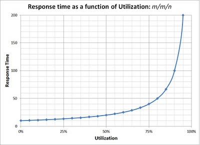
Response time (Latency) vs Utilization [R=1/µ(1-ρ)] for an open system
[from Rules in PAL: the Performance Analysis of Logs tool, figure 1]
With more requests and higher throughput, utilization climbs up to its limit of 100% and latency rises to infinity. The goal of benchmarking is to find the optimal point on that curve, where utilization (or throughput) is highest, with latency at or below the target level. To do that we need to ask questions like:
- What is the maximum throughput of the system when the 99th latency percentile (P99) is less than 10 milliseconds (ms)?
- What is the system latency when it handles 100,000 QPS?
It follows that to measure performance, we need to simulate a workload. The exact nature of that workload is up to the researcher’s discretion, but ideally, it should reflect typical application usage.
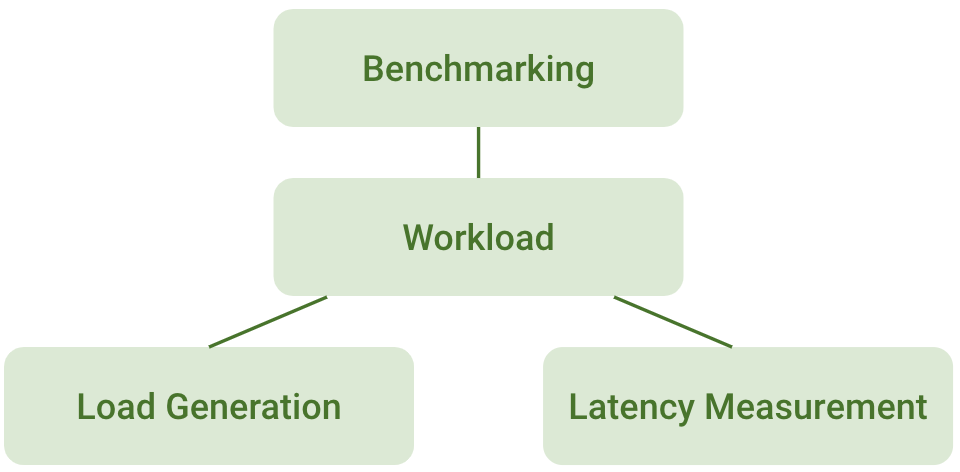
So now we have two problems: generating the load for the benchmark and measuring the resulting latency. This is where the problem of Coordinated Omission comes into play.
Load Generation
The easiest way to create a load is to generate a required number of requests (X) per second:
for (auto i: range{1, X}) {
    std::thread([]() {
      make_request("make a request");
    });
}
The problem comes when X reaches a certain size. Modern NoSQL in-memory systems can handle tens of thousands of requests per second per CPU core. Each node will have several cores available, and there will be many nodes in a single cluster. We can expect target throughput (X) to be 100,000 QPS or even 1,000,000 QPS, requiring hundreds of thousands of threads. This approach has the following drawbacks:
- Creating a thread is a relatively expensive operation: it can easily take 200 microseconds (⅕ ms) and more. It also eats kernel resources.
- Scheduling many threads is expensive as they need to context switch (1-10 microseconds) and share a single limited resource – CPU.
- There may be a maximum number of threads limit in place (see RLIMIT_NPROC and this thread on StackExchange)
Even if we can afford those costs, just creating 100,000 threads takes a lot of time:
#include <thread>

int main(int argc, char** argv) {
  for (int i = 0; i < 100000; i++) {
    std::thread([](){}).detach();
  }
  return 0;
}

$ time ./a.out

./a.out  0.30s user 1.38s system 183% cpu 0.917 total
We want to spend CPU resources making requests to the target system, not creating threads. We can’t afford to wait 1 second to make 100,000 requests when we need to issue 100,000 requests every second.
So, what to do? The answer is obvious: let’s stop creating threads. We can preallocate them and send requests like this:
// Every second generate X requests with only N threads where N << X:

for (int i = 0; i < N; i++) {
  std::thread([]() {
    for (;;) {
      make_request("make a request");
    }
  });
}
Much better. Here we allocate only N threads at the beginning of the program and send requests in a loop.
But now we have a new problem.
We meant to simulate a workload for an open-model system but wound up with a closed-model system instead. (Compare again to Variant 1 and Variant 2 mentioned above.)
What’s the problem with that? The requests are sent synchronously and sequentially. That means that every worker-thread may send only some bounded number of requests in a unit of time. This is the key issue: the worker performance depends on how fast the target system processes its requests.
For example, suppose:
Response time = 10 ms
⟹
Thread sending requests sequentially may send only = 1000 [ms/sec] / 10 [ms/req] = 100 [req/sec]
Outliers may take longer, so you need to provide a sufficient number of threads for your load to be covered. For example:
Target throughput = 100,000 QPS (expect it to be much more in real test)
Expected latency P99 = 10 ms
⟹
1 worker may expect a request to take up to 10 ms for 99% of cases
⟹
We expect 1 worker must be able to send 1,000 [ms/sec] / 10 [ms/req] = 100 [requests/sec]
⟹
Target throughput / Requests per worker = 100,000 [QPS] / 100 [QPS/Worker] = 1,000 workers
At this point, it must be clear that with this design a worker can’t send requests faster than it takes to process one request. That means that we need a sufficient number of workers to cover our throughput goal. To make workers fulfill the goal we need a schedule for them that will determine when a certain worker has to send a request exactly.
Let’s define a schedule as a request generation plan that defines points in time when requests must be fired.
A schedule: four requests uniformly spread in a unit of time:
1000 [ms/sec] / 4 [req] = 250 ms every next request
There are two ways to implement a worker schedule: static and dynamic. A static schedule is a function of the start timestamp; the firing points don’t move. A dynamic schedule is one where the next firing starts after the last request has completed but not before the minimum time delay between requests.
A key characteristic of a schedule is how it processes outliers—moments when the worker can’t keep up with the assigned plan, and the target system’s throughput appears to be lower than the loader’s throughput.
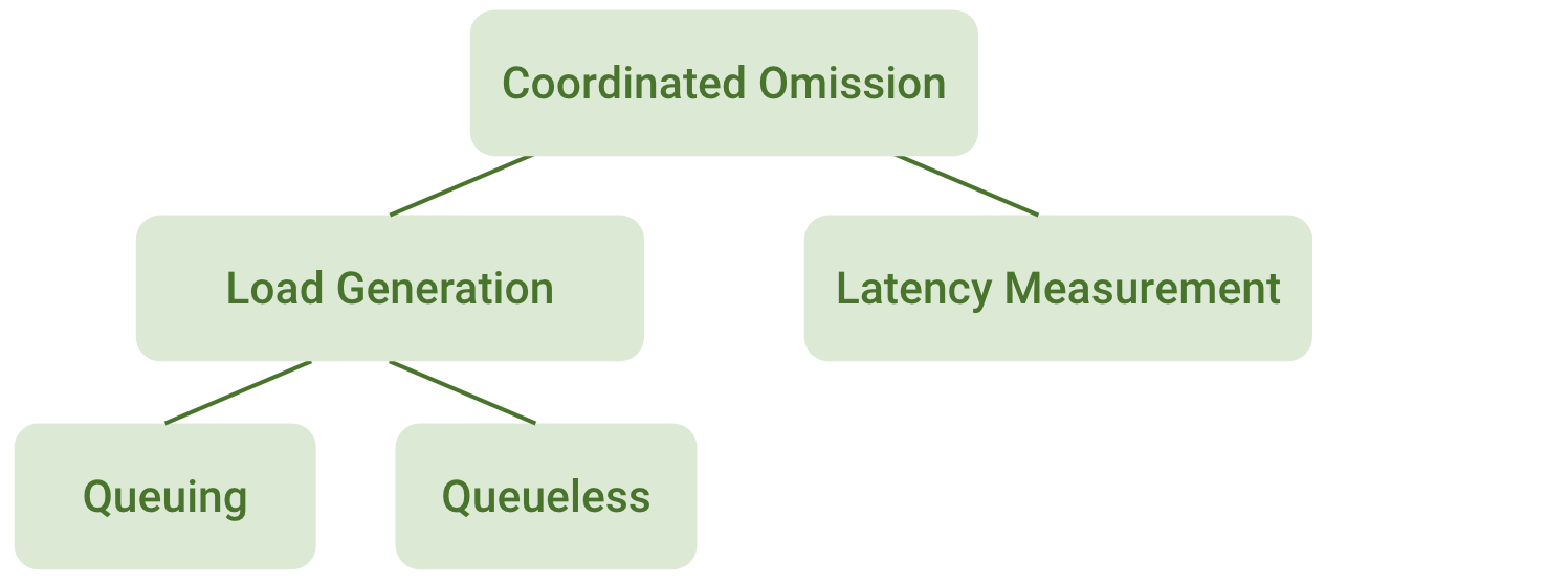
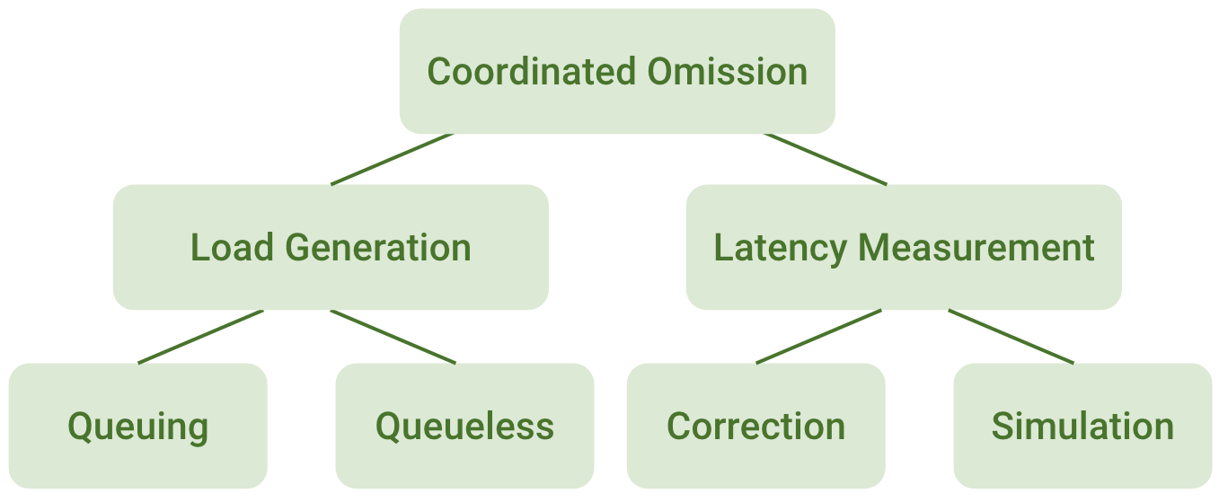
This is exactly the first part of the Coordinated Omission problem. There are two approaches to outliers: Queuing and Queueless.
A good queueing implementation tracks requests that have to be fired and tries to fire them as soon as it can to get the schedule back on track. A not-so-good implementation shifts the entire schedule by pushing delayed requests into the next trigger point.
By contrast, a Queueless implementation simply drops missed requests.
Queueing
The Queuing approach for a static schedule is the most reliable and correct. It is used in most implementations of the benchmark tools: YCSB, Cassandra-stress, wrk2, etc. It does not ignore requests it had to send. It queues and sends them as soon as possible, trying to get back on the schedule.
For example:
Our worker’s schedule: 250ms per request
A request took too long: 1sec instead 250ms
![]()
To get back on track we have to send 3 additional requests
![]()
A static schedule with queuing uses a function that defines when the request need to be sent:
// f(request) = start + (request - 1) * time_per_request

template <class Clock>

Clock::duration next(time_point<Clock> start, milliseconds t, size_t request) {
  return start + (request - 1) * t;
}

template <class Clock>
void wait_next(time_point<Clock> start, milliseconds t, size_t request) {
  sleep_until(next(start, t, request));
}
It also maintains a counter of requests sent. Those 2 objects are enough to implement queuing:
for (size_t worker = 0; worker < workers; worker++) {
    std::thread([=]() {
      for (size_t req = 1; req <= worker_requests; req++) {
        make_request(req);
        wait_next(start, t_per_req, req + 1);
      };
    };
}
This implementation fulfills all desired properties: a) it does not skip requests if it’s missed its firing point; b) it tries to minimize schedule violation if something goes wrong and returns to the schedule as soon as it can.
For example:
Dynamic scheduling with queuing uses a global rate limiter, which gives each worker a token and counts requests as they’re sent.
RateLimiter limiter(throughput, burst = 0);
for (size_t worker = 0; worker < workers; worker++) {
    std::thread([=]() {
      for (size_t req = 1; req <= worker_requests; req++) {
        limiter.acquire(1);
        make_request(req);
      };
    };
}
The drawback of this approach is that the global limiter potentially is a contention point and the overall schedule constantly deviates from the desired value. Most implementations use “burst = 0,” which makes them susceptible to coordination with the target system when system throughput appears lower than the target.
For example, take a look at the Cockroach YCSB Go port and this.
Usage of local rate limiters makes the problem even worse because each of the threads can deviate independently.
Queueless
As the name suggests, a Queueless approach to scheduling doesn’t queue requests. It simply skips ones that aren’t sent on the proper schedule.
Our worker’s schedule: 250ms per request
Queueless implementation that ignores requests that it did not send
![]()
Queueless implementation that ignores schedule
![]()
This approach is relatively common, as it seems simpler than queuing. It is a variant of a Rate Limiter, regardless of the Rate Limiter implementation (see Buckets, Tokens), which completes at a certain time (for example 1 hour) regardless of how many requests are sent. With this approach, skipped requests must be simulated.
RateLimiter r(worker_throughput, burst = 0);

while (now() < end) {
  r.acquire(1);
  make_request(req);
}
Overall, there are two approaches for generating load with a closed-model loader to simulate an open-model system. If you can, use Queuing because it does not omit generating requests according to the schedule along with a static schedule because it will always converge your performance back to the expected plan.
Measuring latency
A straightforward way to measure an operation’s latency is the following:
auto start = now();
make_request(i);
auto end = now();

auto latency = end - start;
But this is not exactly what we want.
The system we are trying to simulate sends a request every [1 / throughput] unit of time regardless of how long it takes to process them. We simulate it by the means of N workers (threads) that send a request every [1 / worker_throughput] where worker_throughput ≤ throughput, and N * worker_throughput = throughput.
Thus, a worker has a [1/N] schedule that reflects a part of the schedule of the simulated system. The question we need to answer is how to map the latency measurements from the 1/N worker’s schedule to the full schedule of the simulated open-model system. It’s a straightforward process until requests start to take longer than expected.
Which brings us to the second part of the Coordinated Omission problem: what to do with latency outliers.
Basically, we need to account for workers that send their requests late. So far as the simulated system is concerned, the request was fired in time, making latency look longer than it really was. We need to adjust the latency measurement to account for the delay in the request.
Request latency = (now() – intended_time) + service_time
where
service_time = end – start
intended_time(request) = start + (request – 1) * time_per_request
This is called latency correction.
Latency consists of time spent waiting in the queue plus service time. A client’s service time is the time between sending a request and receiving the response, as in the example above. The waiting time for the client is the time between the point in time a request was supposed to be sent and the time it was actually sent.
We expect every request to take less than 250ms
1 request took 1 second
![]()
1 request took 1 second; o = missed requests and their intended firing time points
![]()
So the second request must be counted as:
1st request = 1 second
2nd request = [now() – (start + (request – 1) * time_per_request)] + service time =
[now() – (start + (2 – 1) * 250 ms)] + service time =
750ms + service time
If you do not want to use latency Correction for some reason in your implementation, for example because you do not fire the missed requests (Queueless), you have only one option — to pretend the requests were sent. It is done like so:
recordSingleValue(value);
if (expectedIntervalBetweenValueSamples <= 0)
      return;
for (long missingValue = value - expectedIntervalBetweenValueSamples;
      missingValue >= expectedIntervalBetweenValueSamples;
      missingValue -= expectedIntervalBetweenValueSamples) {
      recordSingleValue(missingValue);
}
As in HdrHistogram/recordSingleValueWithExpectedInterval.
By doing that it compensates for the missed calls in the resulting latency distribution through simulation, by adding a number of expected requests with some expected latency.
How Not to YCSB
So let’s try a benchmark of Scylla and see what we get.
$ docker run -d --name scylladb scylladb/scylla --smp 1to get container IP address
$ SCYLLA_IP=$(docker inspect -f "{{range .NetworkSettings.Networks}}{{.IPAddress}}{{end}}" scylladb)to prepare keyspace and table for YCSB
$ docker exec -it scylladb cqlsh
> CREATE KEYSPACE ycsb WITH REPLICATION = {'class' : 'SimpleStrategy', 'replication_factor': 1 };
> USE ycsb;
> create table usertable (y_id varchar primary key,
    field0 varchar, field1 varchar, field2 varchar, field3 varchar, field4 varchar,
    field5 varchar, field6 varchar, field7 varchar, field8 varchar, field9 varchar);
> exit;
build and run YCSB
$ docker run -it debian
# apt update
# apt install default-jdk git maven
# git clone https://github.com/brianfrankcooper/YCSB.git
# cd YCSB
# mvn package -DskipTests=true -pl core,binding-parent/datastore-specific-descriptor,scylla

$ cd scylla/target/
$ tar xfz ycsb-scylla-binding-0.18.0-SNAPSHOT.tar.gz
$ cd ycsb-scylla-binding-0.18.0-SNAPSHOT
load initial data
$ apt install python
$ bin/ycsb load scylla -s -P workloads/workloada \
    -threads 1 -p recordcount=10000 \
    -p readproportion=0 -p updateproportion=0 \
    -p fieldcount=10 -p fieldlength=128 \
    -p insertstart=0 -p insertcount=10000 \
    -p scylla.writeconsistencylevel=ONE \
    -p scylla.hosts=${SCYLLA_IP}
run initial test that does not respect CO
$ bin/ycsb run scylla -s -P workloads/workloada \
-threads 1 -p recordcount=10000 \
-p fieldcount=10 -p fieldlength=128 \
-p operationcount=100000 \
-p scylla.writeconsistencylevel=ONE \
-p scylla.readconsistencylevel=ONE \
-p scylla.hosts=${SCYLLA_IP}
On my machine it results in:
[OVERALL], Throughput(ops/sec), 8743.551630672378
[READ], 99thPercentileLatency(us), 249
[UPDATE], 99thPercentileLatency(us), 238
The results seem to yield fantastic latency of 249µs for P99 reads and 238µs P99 writes while doing 8,743 OPS. But those numbers are a lie! We’ve applied a closed-model system to the database.
Try to make it an open model by setting a target for throughput.
$ bin/ycsb run scylla -s -P workloads/workloada \
    -threads 1 -p recordcount=10000 \
    -p fieldcount=10 -p fieldlength=128 \
    -p operationcount=100000 \
    -p scylla.writeconsistencylevel=ONE \
    -p scylla.readconsistencylevel=ONE \
    -p scylla.hosts=${SCYLLA_IP} \
    -p target ${YOUR_THROUGHPUT_8000_IN_MY_CASE}

[OVERALL], Throughput(ops/sec), 6538.511834706421
[READ], 99thPercentileLatency(us), 819
[UPDATE], 99thPercentileLatency(us), 948
Now we see the system did not manage to keep up with my 8,000 OPS target per core. What a shame. It reached only 6,538 OPS. But take a look at P99 latencies. They are still good enough. Less than 1ms per operation. But these results are still a lie.
How to YCSB Better
By setting a target throughput we have made the loader simulate an open-model system, but the latencies are still incorrect. We need to request a latency correction in YCSB:
$ bin/ycsb run scylla -s -P workloads/workloada \
    -threads 1 -p recordcount=10000 \
    -p fieldcount=10 -p fieldlength=128 \
    -p operationcount=100000 \
    -p scylla.writeconsistencylevel=ONE \
    -p scylla.readconsistencylevel=ONE \
    -p scylla.hosts=${scylladb_ip_address} \
    -p target ${YOUR_THROUGHPUT_8000_IN_MY_CASE} \
    -p measurement.interval=both

[OVERALL], Throughput(ops/sec), 6442.053726728081
[READ], 99thPercentileLatency(us), 647
[UPDATE], 99thPercentileLatency(us), 596
[Intended-READ], 99thPercentileLatency(us), 665087
[Intended-UPDATE], 99thPercentileLatency(us), 663551
Here we see the actual latencies of the open-model system: 665ms per operation for P99 – totally different from what we can see for a non-corrected variant.
As homework I suggest you compare the latency distributions by using “-p measurement.histogram.verbose=true”.
Conclusion
To sum up, we’ve defined coordination omission (CO), explained why it appears, demonstrated its effects, and classified it into 2 categories: load generation and latency measurement. We have presented four solutions: queuing/queueless and correction/simulation.
We found that the best implementation involves a static schedule with queuing and latency correction, and we showed how those approaches can be combined together to effectively solve CO issues: queuing with correction or simulation, or queueless with simulation.
To mitigate CO effects you must:
- Explicitly set the throughput target, the number of worker threads, the total number of requests to send or the total test duration
- Explicitly set the mode of latency measurement
- Correct for queueing implementations
- Simulate non-queuing implementations
For example, for YCSB the correct flags are:
-target 120000 -threads 840 -p recordcount=1000000000 -p measurement.interval=bothFor cassandra-stress they are (see):
duration=3600s -rate fixed=100000/s threads=840Besides coordinated omission there are many other parameters that are hard to find the right values for (for example).
This blog post first appeared on the site of ScyllaDB, sponsor of P99 CONF. Register for P99 CONF to participate in deeply technical discussions by engineers and for engineers who care about P99 percentiles and high-performance, low-latency applications.

