Running Fast and Slow: Experiments with BPF Program Performance

P99 CONF 2023 is now a wrap! You can (re)watch all videos and access the decks now.

ACCESS ALL THE VIDEOS AND DECKS NOW

Editor’s note: The following is a post from PostgreSQL contributor, and Red Hat Software Engineer Dmitrii Dolgov. He spoke at P99 CONF 23 on “Demanding the Impossible: Rigorous Database Benchmarking”: an exploration of how to design an effective database benchmark, including selecting a mode, overcoming technical challenges, and analyzing the results (using PostgreSQL as an example). This article was originally published on his blog. 

Watch Dmitri’sTalk

My own personal white spot regarding BPF subsystem in Linux kernel was always program performance and an overall introspection. Or to formulate it more specifically, I wasn’t sure if there is any difference in how we reason about an abstract program performance versus an BPF program? Could we use the same techniques and approaches?

You may wonder “why even bother” when BPF programs are so small and fast? Generally speaking, you would be right. But, there are cases when BPF programs are not small anymore and they’re placed on the hot execution path (e.g. if we talk about a security system monitoring syscalls). In such situations, even small overhead is drastically multiplied and accumulated, and it only makes sense to fully understand the system performance to avoid nasty surprises.

It seems many other people also would like to know more about this topic, thus I want to share the results of my investigation.

The current state of things

Whenever we analyse performance of some system, it’s always useful to get an understanding of which features and parameters could improve efficiency or make it worse. What is important to keep in mind when writing BPF programs? Looking around I found a couple of interesting examples.

BPF Instruction Set

It turns out that there are several versions of BPF instruction sets available, namely v1, v2 and v3. Unsurprisingly they feature different sets of supported instructions, which could affect how the final program is performing. An example from the documentation:

Q: Why BPF_JLT and BPF_JLE instructions were not
introduced in the beginning?
~~~~~~~~~~~~~~~~~~~~~~~~~~~~~~~~~~~~~~~~~~~~~~~~~~~~~~~~~
A: Because classic BPF didn't have them and BPF authors
felt that compiler workaround would be acceptable.Turned out that programs lose performance due to lack of
these compare instructions and they were added.

This is quite an interesting example of differences between two ISA versions. First, it shows the historical perspective and answers the question of how the versions were evolving over time. Second, it mentions two particular instructions BFP_JLT (jump if less than) and BPF_JLE (jump if less than or equal), which were added into v2. Those are not something you would simply miss among dozens of other instructions, those are basic comparison instructions! For example, you write something like:

if (delta < ts)

In this case, ideally the compiler would like to use BPF_JLT in order to produce an optimal program, but it’s not available in BPF ISA v1. Instead, the compiler has to do some extra mile and reverse the condition using only “jump if greater than” instruction:

; if (delta < ts)
  cmp    %rsi,%rdi
; jump if above or equal
  jae    0x0000000000000068

As soon as we switch BPF ISA to v2 the same code will produce something more expected:

; if (delta < ts)
  cmp    %rdi,%rsi
; jump is below or equal
  jbe    0x0000000000000065

In the case above both versions are equivalent, but if we’re going to compare the value with a constant, the resulting implementation will require one more register load. Interestingly enough I wasn’t able to produce such an example exactly, the compiler was stubbornly generating it only one way around for both versions, but you can find an example in this blogpost. But probably more dramatic changes one can notice between v1 and v3, which adds 32-bit variants of existing conditional 64-bit jumps. Using v1 to compare a variable with a constant will produce the following result, when we have to clean the 32 most-significant bits:

if (delta < 107)

; if (delta < 107)
  15: (bf) r2 = r1
  16: (67) r2 <<= 32 17: (c7) r2 s>>= 32
  18: (65) if r2 s> 0x6a goto pc+3

; if (delta < 107)
  31:   mov    %r13d,%edi
  34:   shl    $0x20,%rdi
  38:   sar    $0x20,%rdi
  3c:   cmp    $0x6a,%rdi
  40:   jg     0x0000000000000048

Whereas using v3 there is no need to do so:

; if (pid < 107) 15: (66) if w1 s> 0x6a goto pc+3

; if (pid < 107)
  31:   cmp    $0x6a,%r13d
  35:   jg     0x000000000000003d

Those two flavours come with different performance characteristics, the former version of the program has to do a bit more work to include the workaround. It also makes the program bigger, using the instruction cache less efficiently. Again, you can get more numbers and the support matrix for Linux and LLVM version in this great blogpost.

Unsurprisingly the default BPF ISA being used normally is the lowest one, v1 also known as “generic”, which means one has to configure it explicitly to use something higher:

$ llc probe.bc -mcpu=v2 -march=bpf -filetype=obj -o probe.od

With clang, one can use -mllvm -mcpu=v2 to do the same.

A few closing notes for this section. Instead of pinning one particular version, one could use probe value to tell the compiler to pick up the highest available ISA for the current machine you’re compiling the program on (see the corresponding part of the implementation). Keep in mind it could be a different machine, not the one which is going to run the program. I’ve got quite curious about this feature, but for whatever reason it’s not always work in those examples I was experimenting with, still defaulting to v1 where v2 was available. And last but not least: the best practice is to always use the latest available instructions set, which is v3 at the moment.

Batching of map operations

Maps are one of the core parts of BPF subsystem, and they could be used quite extensively. One way of making data processing a bit faster (almost independently of the context) is to batch operations. Sure enough, there is something like that for BPF maps as well (for example, a generic support for lookups and modifications). One could use corresponding subcommands:

BPF_MAP_LOOKUP_BATCH
BPF_MAP_LOOKUP_AND_DELETE_BATCH
BPF_MAP_UPDATE_BATCH
BPF_MAP_DELETE_BATCH

and parameters:

struct { /* struct used by BPF_MAP_*_BATCH commands */
    __aligned_u64   in_batch;       /* start batch,
                                     * NULL to start from beginning
                                     */
    __aligned_u64   out_batch;      /* output: next start batch */
    __aligned_u64   keys;
    __aligned_u64   values;
    __u32           count;          /* input/output:
                                     * input: # of key/value
                                     * elements
                                     * output: # of filled elements
                                     */
    __u32           map_fd;
    __u64           elem_flags;
    __u64           flags;
} batch;

An alternative way would be to use libbpf support.

Batching BPF map operations one can save on user/kernel space interaction. The ballpark numbers mentioned in the mailing list were a visible improvement for ~1M record with the batch size 10, 1000, etc. For more details check out the original patch.

Bloom filter map

Continuing on the topic of diverse BPF map features, we find out something very curious among the typical structures like hash, array, queue – a bloom filter map. To remind you of the classical definition:

A Bloom filter is a space-efficient probabilistic data structure
that is used to test whether an element is a member of a set.
False positive matches are possible, but false negatives are not
– in other words, a query returns either "possibly in set" or
"definitely not in set". Elements can be added to the set,
but not removed (though this can be addressed with the counting
Bloom filter variant); the more items added, the larger the
probability of false positives.

Independently of the context, this is a great instrument in our hands, which gives us the possibility to trade off the size of the data structure (we now have to maintain both the hash map and the filter) for more efficient lookups. In the case of BPF, normally checking the bloom filter before accessing the hash map would improve the overall performance, since a costly hash map lookup will be avoided if the element doesn’t exist. We can turn this on when needed by specifying the new map type:

bpf_map_create(BPF_MAP_TYPE_BLOOM_FILTER,
    NULL, 0, sizeof(value), 100, NULL);

Task local storage

But there is more to it! Looking closely, we also find something called task local storage, which gives us another trade-off to play with for one particular use case. Imagine you would like to write a BPF program that works with information about processes. To store anything you would normally create a hash map and use PID as the key, then you realize that large hash maps could be slow. To prevent that (and some other inconveniences) you can use a task local storage instead, which is, surprise surprise, a storage local to the owning task. And this means we’re getting a performance boost accessing such local data on the account of its allocation in a different place. The API is quite straightforward:

ptr = bpf_task_storage_get(&start, t, 0, BPF_LOCAL_STORAGE_GET_F_CREATE);

Interestingly enough,  this feature is not a unique one, There are bpf_local_storage exists for sockets and inodes. For tasks, it was originally implemented only for BPF LSM (Security Audit and Enforcement using BPF), and then extended for tracing programs as well.

BPF program pack allocator

One more topic somewhat related to the memory allocation is the program pack allocator. It turns out that originally every single BPF program was consuming one memory page, no matter how small the program is. Which means that if you end up having a log of such small programs on your server you can observe high instruction TLB (iTLB) pressure in the system, degrading the overall performance. To solve this bpf_prog_allocator was introduced, with the idea to pack programs together on a page when allocating them. This happens transparently, nothing has to be done or configured, and the only thing you may need to think about is whether there are available huge pages on your machines (yes, the packer will try to pack on a huge page as well). For more details check out the LWN article.

BPF 2 BPF

Experimenting with the code layout is generally important for performance, and BPF is not an exception. The thing I didn’t know was that prior to Linux kernel 4.16 and LLVM 6.0 one always had to inline any reusable shared pieces of code in a BPF program:

#ifndef __inline
# define __inline                         \
   inline __attribute__((always_inline))
#endif

static __inline int test_bpf2bpf(void) {}

If we look at this via bpftool this would obviously produce a single chunk of code:

# 0xffffffffc1513a68:
  nopl   0x0(%rax,%rax,1)
  xor    %eax,%eax
  push   %rbp
# [...]

What’s the problem here? The same as with regular code inlining, it’s not always the best choice: it eliminates a call, but increases the code size using instruction cache less efficiently. Fortunately, with modern versions of the kernel you have an option to decide inline or not inline, where the latter will show you two chunks of code with bpftool:

# 0xffffffffc15b810c:
  nopl   0x0(%rax,%rax,1)
  xor    %eax,%eax
# [...]
  callq  0x0000000000002370

# 0xffffffffc15ba47c:
  nopl   0x0(%rax,%rax,1)
  xchg   %ax,%ax
# [...]

How to analyze BPF performance?

In the previous sections we’ve learned there are many interesting techniques on the table to improve the performance of your programs. But how to evaluate them, how to introspect the program and understand what those approaches have changed?

Talking to the compiler

Things are getting started even before the program is executed. What if we ask the compiler for an opinion about the performance of our program? It’s not so strange as it sounds, clang can generate an Optimization Report when compiling a program:

$ clang -O2
    -Rpass=.*
    -Rpass-analysis=.*
    -Rpass-missed=.*
    # ...

The report will contain quite many potential missed optimizations like this one from Global Value Numering pass:

remark: load of type i32
not eliminated [-Rpass-missed=gvn]\

This record says that the compiler found a load operation that potentially could be eliminated. That’s it, the compiler thinks the load is unnecessary, but doesn’t have enough information to prove this for all possible use cases. In my experiments, these types of records were most frequent in the report, and I speculate that this happens because in BPF programs we often pass some values like an execution context via an opaque pointer:

static __always_inline int bpf_example_fn(void *ctx)

In such situations, the compiler has an opportunity to apply certain eliminations, but they are not allowed in case of overlapping pointers (i.e. there are multiple pointers referring to the same memory). This is a hand-waving explanation, but one thing points in its favour – I’ve managed to make the compiler take some number of those missed optimizations by scattering the restrict keyword around:

static __always_inline int bpf_example_fn(void * restrict ctx)

This keyword is the way of letting compiler know that no other overlapping pointers exist.

Aggregated counters

Well, we’re finally running our BPF program. What is the first thing that comes to mind for regular applications at this stage? Right, we check some global counters like uptime and average load. Could we do this for the BPF program?

Fortunately for us, the Linux kernel collects BPF execution counters when instructed to do so:

$ sysctl -w kernel.bpf_stats_enabled=1

Those counters could be read via bpftool:

$ bpftool prog
379: raw_tracepoint [...] run_time_ns 35875602162 run_cnt 160512637

Another hacky way of getting how many times the BPF program was invoked would be to use memory events with perf. Those events allow monitoring access to a certain address in memory, and finding out at which address the BPF program was loaded we can use this feature to get the number of hits (of course you can use the record command instead of trace):

$ cat /proc/kallsyms | grep bpf_prog
[...]
ffffffffc0201990 t bpf_prog_31e86e7ee100ebfd_test [bpf]

$ perf trace -e mem:0xffffffffc0201990:x
[ trigger the BPF program in another session ]
18446744073790.551 ls/242 mem:0xffffffffc0201990:x()

Those numbers are overall counters for the program, which is useful to get some ballpark numbers about the performance to make some sanity check or verify the results obtained using other methods.

Manual instrumentation

The simplest next step in understanding what’s going on inside the BPF program would be to instrument it manually. I mean, nobody will prevent you from modifying your own program, right?

You could write something like this inside the program:

bpf_trace_printk("Timestamp: %lld", ts);

Then fetch the timestamps from either a trace_pipe, or using bpftool:

$ cat /sys/kernel/debug/tracing/trace_pipe
$ bpftool prog tracelog

This is a rather flexible and easy approach. But, unfortunately, it introduces a lot of overhead due to constant user- to kernel space communication, which makes it not quite practical in most situations. If something like this is really needed, instead of using trace_pipe one can introduce the map to buffer data on the kernel side, then periodically read this map.

Top-down approach

Now let’s step back and think. What are the cool kids using to analyse the application performance? For example, the BPF program pack allocator from the previous section, how people have identified that the high iTLB cache pressure is the issue?

Normally there are two options:

• Either one has enough years of experience, making it possible to stare at the screen for an hour and then exclaim “A-ha! We need to check iTLB counters!”
• Or one uses some method to figure out the solution step by step, for example Top-Down approach.

The Top-Down analysis method (see Intel® 64 and IA-32 Architectures Optimization Reference Manual, Appendix B.1 ) helps to identify performance bottlenecks correlating to major functional blocks of modern out-of-order microarchitectures. At the first level, they’re falling into four categories (see more details in Performance analysis and tuning on modern CPUS book):

• Front-End Bound. The modern CPU Front-End main purpose is to efficiently fetch and decode instructions from memory and feed them to the CPU Back-End. Front-End Bound most of the time means the Back-End is waiting for instructions to execute, while Front-End is not able to provide them. An example is an instruction cache miss.
• Back-End Bound. The CPU Back-End is responsible for the actual execution of prepared instructions employing Out-Of-Order engine and store results. Back-End Bound means the Front-End has fetched and decoded instructions, but the Back-End is overloaded and can’t take more to do. An example is a data cache miss.
• Bad Speculation
• Retiring

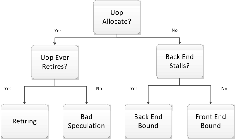
Intel® 64 and IA-32 Architectures Optimization Reference Manual, Appendix B.1

Now, armed with this method, if we face a system with a multitude of BPF programs loaded, we can start categorizing bottlenecks and find out that the system is “Front End Bound”. Digging a few levels deeper we can discover that the reason is iTLB cache pressure, which contributes to the “Front End Bound” load. The only question is how to actually do that?

Well, theoretically perf does support the first level of the Top-Down approach and can collect stats for specified BPF programs:

$ perf stat -b <prog id> --topdown

This machinery works thanks to fentry/fexit attachment points, which allow attaching an instrumentation BPF program at the start/end of another BPF program. It’s worth talking a bit more about this approach, as it works in quite an interesting way. Here is what happens with the BPF program when one has attached an fentry  program to it:

# original program instructions
nopl 0x0(%rax,%rax,1
xchg %ax,%ax
push %rbp
mov %rsp,%rbp
sub 0x20,%rsp
...

# instructions after attaching fentry
callq 0xffffffffffe0096c
xchg %ax,%ax
push %rbp
mov %rsp,%rbp
sub 0x20,%rsp
...

Kernel modifies the BPF program prologue to execute the fentry, which is a remarkably flexible and powerful approach. There are of course certain limitations one has to keep in mind: the target BPF program has to be compiled with BTF, and one cannot attach fentry/fexit BPF programs to another program of the same type (see the verifier for both here and here).

At the end of the day using this approach should give us something like this:

Performance counter stats for 'system wide':

             retiring  bad speculation  frontend bound  backend bound
S0-D0-C0  1  64.2%             8.3%           19.1%          8.5%

Unfortunately, this didn’t work for me. perf was always returning nulls. Digging a bit deeper I’ve noticed that reading the actual perf events was returning empty results. I’m still not sure why (if you have any ideas, let me know).

Trying to figure out if it’s an intrinsic limitation or simply a strange bug in my setup I’ve picked up a bpftool prog profile  command. It’s a great instrument for our purposes which works using fentry/fexit as well, allowing us to collect a certain set of metrics:

bpftool prog profile  [duration ] 

The metrics are one of the following:

• cycles / PERF_COUNT_HW_CPU_CYCLES
• instructions per cycle / PERF_COUNT_HW_INSTRUCTIONS
• l1d_loads / PERF_COUNT_HW_CACHE_L1D + RESULT_ACCESS
• llc_misses per million instructions / PERF_COUNT_HW_CACHE_LL + RESULT_MISS
• itlb_misses per million instructions / PERF_COUNT_HW_CACHE_ITLB + RESULT_MISS
• dtlb_misses per million instructions / PERF_COUNT_HW_CACHE_DTLB + RESULT_MISS

This is a lot of information we could collect doing something like this:

$ bpftool prog profile id  duration 10 cycles instructions

                11 run_cnt
            258161 cycles
             50634 instructions        #     0.20 insns per cycle

Alas, it doesn’t help in the case of the Top-Down approach. As an experiment, I’ve added few perf counters from Top-Down to bpftool and it was able to do the thing and read those counters (the full implementation would be of course much more involving). At the end, it means one can successfully apply the Top-Down approach in case of a BPF program, which is great news.

Profiling of BPF programs

This brings us forward in our quest to understand what’s going on inside a BPF program, but we’re still missing one point. To get the most out of it, we need not only to sample certain events between two points in the program (e.g. fentry/fexit), but also be able to profile the program in general, i.e. sample needed events and attribute them to the corresponding parts of the program. Can we do that?

The question has two parts: Can we do stack sampling, and is it possible to correlate results with the BPF program code? Surely we can do stack sampling, as our BPF program is sort of a “dynamic” extension of the kernel, sampling the kernel will sample the program as well. How to relate it to the code? Fortunately for us perf is smart enough to do that for us if the BPF program builds with BTF support. Here is an example of a perf report collecting cycles without actually retired uops:

$ perf report
  Percent | uops_retired.stall_cycles
          :
          : if (duration_ns < min_duration_ns)
     0.00 :    9f:movabs $0xffffc9000009e000,%rdi
     0.00 :    a9:mov    0x0(%rdi),%rsi
          :
          : e = bpf_ringbuf_reserve(...)
    21.74 :    ad:movabs $0xffff888103e70e00,%rdi
     0.00 :    b7:mov    $0xa8,%esi
     0.00 :    bc:xor    %edx,%edx
     0.00 :    be:callq  0xffffffffc0f9fbb8

From this report we see there is a hot spot of stall events around bpf_ringbuf_reserve, so we may want to look deeper into this helper to understand what’s going on.

But there is a small catch, I’ve mentioned before that we sample our BPF program by sampling the kernel. Now, if you have a relatively busy system that actually does something useful except only running some BPF stuff, you will get a lot of data this way, like tons and tons of samples, only a fraction of which is actually of any interest to you. To make it manageable one can try to capture only the kernel part of stacks, maybe isolate the BPF program on a single core if the environment allows that, but it still would be quite a lot.

At some point, I realized there is a –filter perf option to do an efficient filtering of the data using Intel PT, and in theory one could do something like this:

# with the program name
$ perf record -e intel_pt// --filter 'filter bpf_prog_9baac7ecffdb457d'

# or with the raw address
$ perf record -e intel_pt// --filter 'start 0xffffffffc1544172'

Unfortunately, it seems this is not supported for BPF:

failed to set filter "start 0xffffffffc1544172" on event intel_pt// with 95 (Operation not supported)

Nevertheless, having both the Top-Down approach and profiling for BPF opens quite interesting opportunities. Let’s take a look at the previous example with the program allocator packer. The idea was to reduce overhead (in the form of iTLB pressure) via packing BPF programs together on a page, without knowing anything else about those programs. Now let’s take one more step forward and try to apply this in the real world, where quite often it’s not a single BPF program, but a chain of programs processing a different part of an event and connected together via tail calls. Packing such programs together may produce a situation when some more frequently invoked (hot) pieces are located on the same page with less demanded (cold):

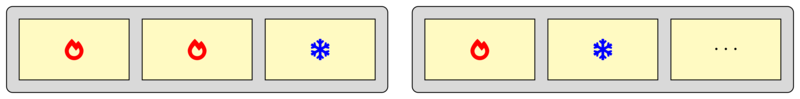
Such placement would not be as optimal as having most of the hot programs together, increasing the number of pages that have to be frequently reached to execute the full chain of processing. But to define an “optimal” placing, we need to know what are the hot and cold programs, so we end up applying both approaches mentioned above: First identify the largest bottleneck (iTLB), then use profiling to find out how to pack everything more efficiently. Note, that nothing like this is of course implemented – although one can try to manipulate the order in which programs are loaded to influence the final placement.

Modeling of BPF programs

We were talking about a great many details that could affect the performance of a BPF program. There are even more factors (not necessarily BPF only) we were not talking about. In this complex picture of many actors interacting in different ways, how to get a prediction about the performance of your program? Intuition may fail you because sometimes improvements in one area reveal an unexpected bottleneck in another. One can benchmark the program under the required conditions, but often it’s resource intensive to cover many cases. And obviously it could be done only when the program is already written, and it’s even more problematic to fix a performance issue. The last option left on the table is to model the program behaviour and experiment with the model instead of an actual implementation. This would be much faster, but the catch is that the results are only as good as the model allows it.

“The Thrilling Adventures of Lovelace and Babbage”, Sydney Padua, 2015

Nevertheless, even the simplest models could give very valuable feedback. Inspired by the article above from Marc Brooker I wanted to see what it takes to simulate a simple BPF program execution. As an example, I took runqslower program from the Linux kernel repository, that uses a BPF program to trace scheduling delays. Its implementation was recently switched to use task local storage instead of a hash map, which is an interesting study case. To make it even simpler for my purposes I’ve tried to simulate not the full difference between two implementations (task local storage is simply faster), but how much effect memory access in the hash map (slower with more elements in the map) has on the final performance.

Simply, the simulation goes like this:

• The program behaviour is specified via a state machine.
• Transitions between states are handled in the event loop.
• Every transition is associated with a certain “resource” consumed, in our case simply execution time.
• Initial state as well as execution time for every state are specified as random values with a distribution of a certain type.

The state machine from the task point of view looks like this:

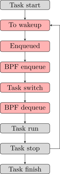
• When the task is ready to be executed, it’s being added into a scheduler queue.
• The BPF program adds a record into the hash map containing the PID and the timestamp of the new task.
• The task spends some time in the queue, then gets dequeued to run for a slice of time.
• The BFP program picks up the recorded PID and timestamp to report them.
• The task finishes the time slice, then waits to get enqueued again.

Every event from the state machine needs to have an associated latency distribution, which would tell how much time the system has spent in this state. For simplicity, I’ve taken the normal distribution with the following mean/stddev:

• Time spent in the queue: ~4/1
• Process enqueue in the BPF program: ~400/10
• Process dequeue in the BPF program: ~200/10
• Time slice for the task to run: 3000000 (sched_min_granularity_ns)/1000
• Report using bpf_perf_event_output helper: ~24/8

Now a warning. No, not like this – a WARNING: It’s hard to come up with real numbers – pretty much like in quantum physics if we try to measure something it will be skewed. It means that the values above should be considered only as an approximation, roughly measured on my laptop under certain conditions (to be more precise when runqslower measures latencies slower than 100ns and some processes are getting spawn in a loop). This is the part when we do quality trade-offs about the model.

Another point is the distribution type. Of course, using normal distribution is unrealistic, as most likely those have to be some long-tailed distribution if we’re dealing with a queue-like process or an exponential distribution if some events are happening independently at a certain constant average rate. This is one of the parts that makes our model “simple”.

None of those points stops us from experimenting or should prevent you from improving the model to be more realistic.

We encode a few more important factors in the model, together with the state machine itself:

• First, without some type of process contention, it’s not going to be interesting. To represent that lets introduce an additional overhead, which will be linearly growing with the number of processes running on a CPU code starting from a certain threshold. This would be similar to the saturation, when the execution queue is full. It means the latency of running the process would be a random variable taken from normal distribution normalized by contention level. The latter one is simplified to the CPU load when it’s higher than a certain constant (in the implementation CPU load is expressed via number of events happening on the core, and I’m using 4 as the threshold, probably instinctively thinking about the pipeline width of modern CPUs).
• Second, to represent the difference between a hash map and a task local storage we add another type of overhead depending on the size of hash map. The constants here are pretty arbitrary, I’ve implemented it as the map size divided by 2¹⁰ in the second degree.

Here is what my final implementation looks like: runqslower-simulation. Warning, it’s the lowest quality Haskell code you’ve seen, riddled with bugs and inconsistencies, but I hope it shows the point. To summarize:

• We record time spent in various states, taking into account all the quirks like contention in the system.
• Sum all the latencies related to BPF events (plus reporting if the value we want to record is higher than the threshold set for runqslower).
• Sum all the processing latencies.
• To calculate the overhead of the BPF program we compare these two sums to see which portion of the runtime was spent doing bookkeeping.

Having everything in place and the model defined, now let’s talk about the input and the output. The initial conditions to start the simulation are completely up to us, so let’s set it to a bunch of processes starting together and doing something for a certain amount of time. The output of the model for us would be records of time spent doing the actual job (positive payload) versus time spent running the BPF parts (bookkeeping overhead). The results would look like this:

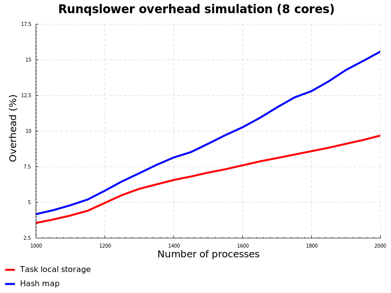
As expected, on the graph we observe that hash map performs slower than task local storage, and even can derive at which point in time this difference becomes significant. The dynamics of this model could be directed via number of processes and their lifetime, producing results in the phase space that are either converging to null (when there is not enough work to do for BPF, and process runtime dominates), exploding into the infinity (when there are too many short-lived processes and BPF overhead is getting more and more significant), or oscillating around certain value (when both BPF and process runtime are balancing each other, producing stable system).

Summary

In this blog post, we were talking a great deal about the performance of BPF programs, the current state of things and various analysis approaches starting from simplest to most intricate. I’m glad to see that the BPF subsystem recently started to provide a flexible set of features to tune efficiency for different use cases, and maturing introspection techniques. Those experiments I’ve conducted along the lines were driven mostly by curiosity, but I hope the results will help you to reason about your BPF programs with more confidence.

Acknowledgments

Huge thanks to Yonghong Song, Joanne Koong and Artem Savkov for reviews and commentaries!

Watch Dmitry’s talk from P99 CONF 23

Here’s a look at what Dmitry presented at P99 CONF 23…

It’s easy to conduct a misleading benchmark, and notoriously hard to design a correct and rigorous enough one. Have you ever asked why?

In this talk, we will discuss database benchmarking using the example of PostgreSQL:

• What is the best model to think about benchmarking?
• What are the typical technical challenges?
• What level of PostgreSQL details do you need to know to not mess up and draw the right conclusions?
• How to analyze the results, and what does it have to do with statistics?

Watch Dmitri’sTalk